Finding my wife in a 3-hour tennis broadcast with face recognition

One reference clip, 3h50m of Wimbledon footage, and the boring engineering that made a GPU pipeline trustworthy

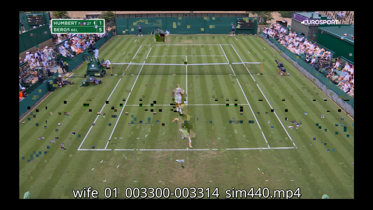
My wife was in the crowd at Wimbledon, and I was at home watching the livestream. At some point, the Eurosport broadcast cut to her in the stands.

I wanted to grab a short screen-recording clip so I could send it to her while she was still in London. I managed to catch one appearance by hand, but after the match was over I had the full recording: 3 hours and 50 minutes, 1920×1200, 30fps, about 12GB.

I knew she had appeared several more times throughout the match, but I did not want to spend an afternoon dragging a scrubber bar back and forth trying to find every crowd shot.

So I reframed it. This was not a “watch the video carefully” problem. It was a face-recognition problem: I had one reference clip of a face, and I wanted every timestamp where that face appeared, plus a few seconds of padding, cut into separate clips.

The surprising part was that the machine-learning side was not the hard part. I did not train a model, label a dataset, tune a neural network, or do anything especially clever. I used an existing face-recognition model and glued the pieces together. The things that actually mattered were much more practical: making sure the GPU was really being used, choosing a threshold I could trust, and cutting video without creating broken clips.

The pipeline

The shape is boring on purpose:

1. Build a reference embedding of her face from the clip I already had.
2. Sample the full video at 2 frames per second.
3. Detect every face in each sampled frame.
4. Compare each detected face to the reference.
5. Log the timestamp and similarity score of every match.
6. Cluster nearby matches into appearance windows.
7. Add padding and cut the clips.

For the face-recognition model I used InsightFace's buffalo_l, which combines RetinaFace for face detection with ArcFace embeddings for recognition.

I picked it because I did not need a custom model. I needed a reliable, off-the-shelf pipeline that could detect faces in broadcast footage and turn each face into an embedding I could compare with cosine similarity. buffalo_l is a larger InsightFace model pack, so it is not the lightest option, but for a one-off scan on an RTX 4090 I cared more about robust matching than squeezing out every last frame per second.

For the reference, I started from the clip I had already found manually. I detected her face across that clip, kept the matches above a loose threshold, and averaged those embeddings into a single reference vector. That gave me a more stable representation than relying on one frame: slightly different angles, lighting, and expressions, but the same identity.

Frames came out of ffmpeg piped as raw bgr24:

ffmpeg -i match.mp4 -vf fps=2 -f rawvideo -pix_fmt bgr24 -

Python read each frame, ran detection, and computed cosine similarity between every detected face and the reference embedding. Anything above a low floor was logged with its timestamp, score, and a saved crop.

Sampling at 2fps meant I could miss a crowd shot shorter than half a second, but for this broadcast that was a reasonable trade-off. Crowd cuts lasted long enough that I did not need to process all 414,000 frames.

Gotcha 1: the GPU that wasn't

The first thing that bit me was the most embarrassing, and probably the most common.

I installed onnxruntime-gpu, prepared the model with CUDAExecutionProvider first in the provider list, and it ran.

It just ran on the CPU.

Two things were wrong. First, InsightFace pulls in the CPU-only onnxruntime package as a dependency, and having both installed meant the CPU build was being used. Second, even after fixing that, the CUDA provider silently fell back because the CUDA userspace libraries were not on the path.

ONNX Runtime does not necessarily fail loudly when a provider cannot initialise. It can log a warning and quietly use the next provider in the list.

The lesson is a one-liner you should paste into every GPU inference script:

print(app.models["detection"].session.get_providers()[0])

Assert the provider you are actually running on. Do not assume that “I asked for CUDA and it did not crash” means you got CUDA.

Once the libraries were sorted, detection throughput went from around 11fps to around 25fps, and the full 3h50m scan finished in 18.5 minutes: 27,606 sampled frames and 481 raw matches.

Gotcha 2: trust the eyes, not only the number

481 matches does not mean 481 appearances. It only means 481 sampled frames where some detected face scored above a deliberately low similarity floor.

The real question was where to draw the line.

Looking at the score distribution, there was a clear noise floor. Between 0.20 and 0.25, the count dropped from 481 to 237. Most of the low-scoring matches were other faces in the crowd. Above that, the count declined more smoothly.

But I did not want to pick a threshold just because the chart looked plausible. So I built a contact sheet: the single best face crop from each candidate appearance, laid out in a grid and labelled with its score.

That one image settled it.

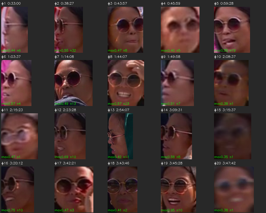
At a 0.35 threshold I got 20 appearance windows, and she was visible in all 20. No false positives. Her round sunglasses made the visual check especially easy: once the candidates were on a contact sheet, the correct matches were obvious.

When I dropped the threshold to 0.30 to try to “catch everything,” the extra windows were tiny, dark, blurry faces with no sunglasses at all. Exactly the kind of noise the distribution suggested.

The contact sheet turned a threshold debate into a two-second visual check.

This is also where the real-world context mattered. A more average-looking face in a Wimbledon crowd, with many people wearing sunglasses and summer clothes, would have been harder to separate cleanly. The model gave me similarity scores, but the final confidence came from looking at the results.

Gotcha 3: cutting on the wrong frame

With 20 windows found, I merged nearby hits, padded each side by 5 seconds, and cut the clips.

My first attempt used stream copy:

ffmpeg -ss <start> -to <end> -c copy out.mp4

Fast, lossless, and wrong.

The first second of several clips was a pixelated mess of drifting macroblocks. The reason is that H.264 frames often reference earlier frames. If you cut in the middle of a group-of-pictures, the first frames in your new clip may depend on a keyframe that is no longer there. The decoder has to guess until it reaches the next usable keyframe.

The fix was to re-encode each clip so it started cleanly. On the 4090, using NVENC, this was almost free: all 20 clips were re-encoded in 41 seconds, visually lossless, with the artifacts gone.

The result

The final output was 20 short clips, one per appearance, with 5 seconds of padding on each side. Each filename included the timestamp and match confidence, so I could quickly scan what had been found.

Appearance #7, from 1:14:08 to 1:14:24, similarity 0.49.

The face-recognition part worked because the hard ML problem had already been solved by someone else. I did not build a model. I used a good existing one.

The part that made the project actually usable was the boring engineering around it:

• verify that the GPU is really being used;
• inspect candidate matches visually instead of trusting a number blindly;
• understand enough about video encoding to cut clips correctly.

That was the useful lesson for me.

The model found the face. The engineering made the result trustworthy.